Rotations in Space: Euler Angles, Matrices, and Quaternions

This notebook demonstrates how to use clifford to implement rotations in three dimensions using euler angles, rotation matices and quaternions. All of these forms are derived from the more general rotor form, which is provided by GA. Conversion from the rotor form to a matrix reprentation is shown, and takes about three lines of code. We start with euler angles.

Euler Angles with Rotors

A common way to parameterize rotations in three dimensions is through Euler Angles.

“Any orientation can be achieved by composing three elemental rotations. The elemental rotations can either occur about the axes of the fixed coordinate system (extrinsic rotations) or about the axes of a rotating coordinate system, which is initially aligned with the fixed one, and modifies its orientation after each elemental rotation (intrinsic rotations).” -wikipedia

The animation below shows an intrinsic rotation model as each elemental rotation is applied. Label the left, right, and vertical blue-axes as \(e_1, e_2,\) and \(e_3\), respectively. The series of rotations can be described:

1. rotate about \(e_3\)-axis
2. rotate about the rotated \(e_1\)-axis, call it \(e_1^{'}\)
3. rotate about the twice rotated axis of \(e_3\)-axis, call it \(e_3^{''}\)

So the elemental rotations are about \(e_3, e_{1}^{'}, e_3^{''}\)-axes, respectively.

from IPython.display import Image,SVG
Image(url='_static/Euler2a.gif') # taken from wikipedia

Following Sec. 2.7.5 from “Geometric Algebra for Physicists”, we first rotate an angle \(\phi\) about the \(e_3\)-axis, which is equivalent to rotating in the \(e_{12}\)-plane. This is done with the rotor

\[R_{\phi} = e^{-\frac{\phi}{2} e_{12}}\]

Next we rotate about the rotated \(e_1\)-axis, which we label \(e_1^{'}\). To find where this is, we can rotate the axis,

\[e_1^{'} =R_{\phi} e_1 \tilde{R_{\phi}}\]

The plane corresponding to this axis is found by taking the dual of \(e_1^{'}\)

\[I R_{\phi} e_1 \tilde{R_{\phi}} = R_{\phi} e_{23} \tilde{R_{\phi}}\]

Where we have made use of the fact that the psuedo-scalar commutes in G3. Using this result, the second roation by angle \(\theta\) about the \(e_1^{'}\)-axis is then ,

\[R_{\theta} = e^{\frac{\theta}{2} R_{\phi} e_{23} \tilde{R_{\phi}}}\]

However, noting that

\[e^{R_{\phi} e_{23} \tilde{R_{\phi}}} =R_{\phi} e^{e_{23}} \tilde{R_{\phi}}\]

Allows us to write the second rotation by angle \(\theta\) about the \(e_1^{'}\)-axis as

\[R_{\theta} = R_{\phi} e^{\frac{\theta}{2}e_{23}} \tilde{R_{\phi}}\]

So, the combonation of the first two elemental rotations equals,

\begin{align*} R_{\theta} R_{\phi} &= R_{\phi} e^{\frac{\theta}{2}e_{23}} \tilde{R_{\phi}} R_{\phi} \\ &= e^{-\frac{\phi}{2} e_{12}}e^{-\frac{\theta}{2} e_{23}} \end{align*}

This pattern can be extended to the third elemental rotation of angle \(\psi\) in the twice-rotated \(e_1\)-axis, creating the total rotor

\[R = e^{-\frac{\phi}{2} e_{12}} e^{-\frac{\theta}{2} e_{23}} e^{-\frac{\psi}{2} e_{12}}\]

Implementation of Euler Angles

First, we initialize the algbera and assign the variables

from numpy import e,pi
from clifford import Cl

layout, blades = Cl(3)   # create a 3-dimensional clifford algebra

locals().update(blades) # lazy way to put entire basis in the namespace

Next we define a function to produce a rotor given euler angles

def R_euler(phi, theta,psi):
    Rphi = e**(-phi/2.*e12)
    Rtheta = e**(-theta/2.*e23)
    Rpsi = e**(-psi/2.*e12)

    return Rphi*Rtheta*Rpsi

For example, using this to create a rotation similar to that shown in the animation above,

R = R_euler(pi/4, pi/4, pi/4)
R

0.65328 - (0.65328^e12) - (0.38268^e23)

Convert to Quaternions

A Rotor in 3D space is a unit quaternion, and so we have essentially created a function that converts Euler angles to quaternions. All you need to do is interpret the bivectors as \(i,j,\) and \(k\)’s. See the page “Interfacing Other Mathematical Systems”, for more on quaternions.

Convert to Rotation Matrix

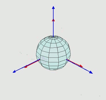
The matrix representation for a rotation can defined as the result of rotating an ortho-normal frame. Rotating an ortho-normal frame can be done easily,

A = [e1,e2,e3]          # initial ortho-normal frame
B = [R*a*~R for a in A] # resultant frame after rotation

B

[(0.14645^e1) + (0.85355^e2) + (0.5^e3),
 -(0.85355^e1) - (0.14645^e2) + (0.5^e3),
 (0.5^e1) - (0.5^e2) + (0.70711^e3)]

The components of this frame are the rotation matrix, so we just enter the frame componenets into a matrix.

from numpy import array

M = [float(b|a) for b in B for a in A] # you need float() due to bug in clifford
M = array(M).reshape(3,3)

M

array([[ 0.14644661,  0.85355339,  0.5       ],
       [-0.85355339, -0.14644661,  0.5       ],
       [ 0.5       , -0.5       ,  0.70710678]])

Thats a rotation matrix.

Convert a Rotation Matrix to a Rotor

In 3 Dimenions, there is a simple formula which can be used to directly transform a rotations matrix into a rotor. For arbitrary dimensions you have to use a different algorithm (see orthoMat2Verser() in clifford.tools). Anyway, in 3 dimensions there is a closed form solution, as described in Sec. 4.3.3 of “Geometric Algebra for Physicists”. Given a rotor \(R\) which transforms an orthonormal frame \(A={a_k}\) into \(B={b_k}\) as such,

\[b_k = Ra_k\tilde{R}\]

\(R\) is given by

\[R= \frac{1+a_kb_k}{|1+a_kb_k|}\]

So, if you want to convert from a rotation matrix into a rotor, start by converting the matrix M into a frame \(B\). (You could do this with loop if you want.)

B = [M[0,0]*e1 + M[1,0]*e2 + M[2,0]*e3,
     M[0,1]*e1 + M[1,1]*e2 + M[2,1]*e3,
     M[0,2]*e1 + M[1,2]*e2 + M[2,2]*e3]
B

[(0.14645^e1) - (0.85355^e2) + (0.5^e3),
 (0.85355^e1) - (0.14645^e2) - (0.5^e3),
 (0.5^e1) + (0.5^e2) + (0.70711^e3)]

Then implement the formula

A = [e1,e2,e3]
R = 1+sum([A[k]*B[k] for k in range(3)])
R = R/abs(R)

R

0.65328 - (0.65328^e12) - (0.38268^e23)

blam.